
Can better data let you make better decisions..?
Maybe yes, with Excel text formulas you can analyze data effectively.
Every day your business will generate millions of lines of data, and most of the times your data will not be in a structured way, even the best technology in the world cannot give you ready-made data to support your decision-making process.
I think that is the reason why we’re so heavily dependent on MS Excel from simple to complicated analysis.
Here is a tutorial that will help you understand various excel text formulas and how to use them effectively to analyze your data systematically.
List of excel text formulas with examples:
1) CONCATENATE:
Formula that joins two or more text strings, maximum up to 255
Syntax: CONCATENATE (text1, [text2],…)
Text1: First text that you want to add
Text2: Second, Third, Fourth, and so on up to 255
Example#1: In my example below, I’ve first names in Column A and Second names in Column B, I just want to add both the names together so that my data will look better for my analysis.
To do so we can write a simple formula like below.
=CONCATENATE(A2,”.”,B2)
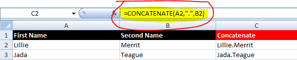
In my above formula, A1 & B2 is my data cells & “.“ codes used to add single period (dot) to differentiate first & second name.
Similar to this you can also add any type of symbols like , – * etc.
Example #2 since we have both first & second names in column “C”, and now we would like to convert them to an E-mail id by adding “@xyz.com” at the end.
Here is a formula:
=CONCATENATE(C2,”@xyz.com”) = Lillie.Merrit@xyz.com
I’ve taken column C2, because that is where we have added formula to combine first & second names.
“@xyz.com” : Its an e-mail extension, it’s quite similar to any corporate e-mail id like @hp.com, @oracle.com and so on.
Please note, you can add any type of text using concatenate formula, but the catch here is, it should be enclosed with codes like this “your text”.
Example #3: Now we have e-mail id in column “D”, with that we would like to send out e-mail to all the people, but the challenge here is you need to copy paste all the emails side by side for a mass communication.
Indeed you can use formula like below to quickly create mailing list; we have two steps in this formula
Step1: Adding first and second e-mail id together in column “E2”
=CONCATENATE(D2,”;”,D3)
Step2 : Second formula to join text string in E2 with D4 so that when we drag down till end you will have email list created automatically.
=CONCATENATE(E2,”;”,D4)

E2 : is my range where I already added first & Second email id’s
D4 : is my next email id that I want to add to my mailing list
Note: please do not select D3 as your range for second formula, because it will add second email ID twice.
For your mailing list, just go to last row of your data and just do a copy paste in your outlook.
Also read: 4 MS Excel alternatives to analyse data
2) EXACT ()
It’s a formula that compares two strings and tell you whether two strings are same or not, if it’s same then it will return ‘True” if not you’ll have ‘False’.
Syntax: EXACT(text1, text2)
Please note: Exact is case sensitive, hence be careful when you comparing
Example #4 In this example I’m just comparing salesman names to check data accuracy from two different sources.
Here is a formula:
=EXACT(A2,B2)
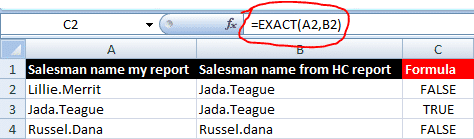
As per above I’m just simply looking whether salesman name in Column A matches with exact row in Column B.
In cell C2 I have ‘false’ because two names are not same and in cell C4 I’ve again false, but this name is same but second name first letter is in lower case “Russel.dana”.
3) FIND()
Formula that will return first occurrence position of your search string.
Syntax: FIND(find_text, within_text, [start_num])
find_text: text string that you’re looking for
within_text: target text, basically it’s a text in which you’re searching
[start_num]: you can specify your starting point from where you want to check, and it’s an optional value
Example #5 In this exercise we have a employee name as below, you are required to find out starting position of employee second name.
=FIND(“.”,”Barry.Chee”) =6
I’m basically looking for a period in the above text because that is the only point where you can see starting position of employee last name.
Please note,* Find & Search functions looks identical in most of the cases, but they are not. You can refer find vs search for further understanding.
4) LEFT ()
Formula to extract certain number of letters from a given text string.
Syntax: LEFT(text, [num_chars])
text: your actual text
[num_chars]): we can specify number of characters that you want to extract
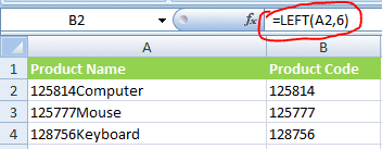
Example# 6 In this exercise we have a list of products with product code prefixed to it, now we would like extract only product code to a separate column so that I can use it for my data analysis. To do so you can write simple formula like below.
=LEFT(A2,6)
A2 : is my text
6 : we want to extract only first 6 digits from left side of the text string
Combination of Left & Find formulas:
You can actually do even more complicated analysis by combining two or more formulas, just to give a flavor, here is my another example.
Example# 7 In this example we have Employee number followed by employee name in one column, now you are required to extract only employee number to a different column.
The problem here is, employee number does not have a specific number of digits, few employees have 3 digit code few has 5 digits and few has 7 digits.
Basically I’ll split this formula in to two parts, first one is to identify number of digits to extract, to do so you can use FIND function like below.
Step 1:
FIND(” “,A2) = 7
In find_text section I’ve added open and closed code to indicate, we want to search for blank space in our text string.
A2 is our original text
With this formula you’ll be able to identify number of letters to extract based on a blank space.
Step 2:
LEFT(A2,FIND(” “,A2))
In this step I‘ve added LEFT formula & selected A2 as my original text.
If you notice clearly I’ve added FIND formula to identify number of digits to extract, so the result will be exactly what we want.

5) LEN ()
The formula to identify a number of letters in a given text string.
Syntax: LEN(text)
LEN is one of the widely used formula by most of the excel experts, it’s very simple and works like champ.
Example# 8 In this example we have employee e-mail id’s in one column, with those you want to see how many letters are there in each employee e-mail id.
Here is a formula:
LEN(“Lillie.Merrit@xyz.com”) = 21
Note: Len function will also count blank spaces
Ok, my above example is simple & straight forward, with that you cannot achieve anything. But when you combine LEN formula with any other formulas then you can have grater advantages.
Here is my example to show how we can use Len with Left formula to extract specific text strings.
Example # 9 We use same employee e-mail id’s from the above example, now we want to extract only employee name from e-mail id.
=LEFT(A2,LEN(A2)-8)
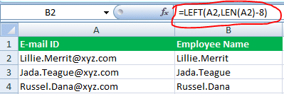
A2 is our text, in this case its employee e-mail id
LEN(A2) : we are basically counting number of digits in employee e-mail id
-8 : it’s a count of letters that we don’t want to have it in our new column (in all the e-email id’s we have “@xyz.com” in common, so when I count these letters its around 8)
So, basically I’m instructing Len formula to count the total number of digits and then subtract 8 digits from it, so that the remaining letters will be extracted to a new column.
6) LOWER ()
The formula to convert any text to a lower case.
Syntax: LOWER(text)
Example #10 In this example, we have a upper case text as mentioned below, now you want convert that to a lower case. To do so you can use Lower formula like this.
=LOWER(“HELLO JAY GOOD MORNING..!!”) = hello jay good morning..!!
7) MID ()
It’s a formula to extract middle value of a text string based on the user requirement.
Syntax: MID(text, start_num, num_chars)
text: the data from where you want to extract certain number of letters
start_num: user input based on starting position of your required text
num_chars: number of characters that you want to extract from your text
Example #11 In my example we’ve a product list prefixed with Company name, Product name and the Product code, you are required to extract only product name to a different cell.
=MID(A1,8,40)

A1 : is our data range
8 : Starting position of your desired value, in this case we have “Ballon” 6 letters and 1 space = 7. So starting position would be 8.
40: Number of letters in our product, it may vary from product to product hence I’ve given 40 as a maximum limit.
8) PROPPER ()
It’s a formula to convert first letter in each word to an upper case and rest all to be in lower case.
Here is a simple formula that will convert improper text to proper one:
=PROPER(“HELLO JaY GOoD MoRnINg..!!”) = Hello Jay Good Morning..!!
*Also read: Advanced Vlookup Tutorial
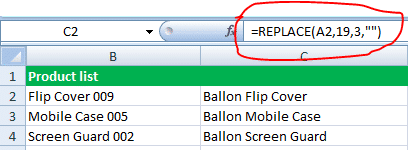
9) REPLACE ()
The formula to replace a certain portion of text in a sentence.
Syntax: REPLACE(old_text, start_num, num_chars, new_text)
old_text : Your actual text
start_num : From which position or letter you want to replace
num_chars : How many characters that you wish to replace
new_text : And the next text that you want to add
Example#13: I’ve used same data from example #11. In this case we don’t want to have product code, so we have to replace that with none.
**=REPLACE(A1,19,3,””) **
10) REPT()
The formula used to repeat a text or symbol based on the number of times that a user wants.
Just to give you a simple example, we want repeat * symbol 10 times in a cell, to do so we can write a formula like this.
=REPT(“*”,10) = **********
REPT formula is very useful to create line graphs within cells based on user customization
11) SEARCH ()
A formula to identify the position of a user-defined text string within a text.
Syntax: SEARCH(find_text,within_text,[start_num])
find_text: It’s a text, letter or symbol that you want to locate
within_text: in which destination text you want to have a look
[start_num]: is an optional value through which you can define your starting point to perform a search in a string.
Example #14: We’ve a list of employee names in column A1, you are required to find out starting position of employee last name.
A2 = Lillie Merrit
=SEARCH(” “,A2) = 7
In my above formula, search value is a blank space, hence I’m using “ “ codes, and A2 is our destination text.
7 is a result for the above formula, which means employee last name in A2 starts from 7th position.
Another variant: what if you have multiple spaces in your text string..? for example same employee name is also have an employee ID at the end.
Here is a formula by defining a starting number of search position.
=SEARCH(” “,E2,SEARCH(” “,E2)+1)
I’ve added another Search formula to identify first blank space position, and then added +1 to define starting number for second blank space.
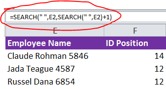
For example, based on my first formula you’ll get “7” i.e. your first blank space position, So if I add +1 it will be 8 in our starting number section.
So, we are basically instructing excel to find blank space from 8th position of our text.
12) RIGHT ()
A formula to extract a certain number of characters from the right side of the text string.
Syntax: RIGHT(text,[num_chars])
Text: user defined text
[num_chars]: Number of letters that you want to extract.
Example #15: In this example we have employee full name in column A, you are required to extract only employee last name to column B.
Text in A2 : Lillie.Merrit
=RIGHT(A2,6) = Merrit
A2 is my text
6 is a number of letters that you want to extract.
Another variant:
What if you don’t know how many letters to extract, can we do something..? Yes indeed.
Here is a formula that can automatically identify last name and extracts to a new cell.
=RIGHT(A2,LEN(A2)-SEARCH(“.”,A2))
To define number of characters, I’ve used two different formulas here.
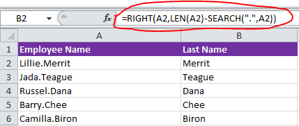
LEN function to identify the total number of letters in a text string and Search formula to find out a specific text location based on my own definition.
So, basically, we are deducting the total number of characters until “.”or “period” from our text.
13) SUBSTITUTE ()
A formula to replace certain portions of text, symbol or numbers in an original text based on user input.
Syntax: SUBSTITUTE(text, old_text, new_text, [instance_num])
Text : your actual text
old_text : your old text that you want to replace
new_text : new text as per your requirement
[instance_num] : you can define your instance number like first occurrence, second third and so on.
Example #16: In this example, we have same employee names in Column A, whereas you are required to replace period between first and second name with underscore “_”.
Text in A2 : Lillie.Merrit
=SUBSTITUTE(A2,”.”,”_”) = Lillie_Merrit
A2 is our actual text
“.” is our original differentiator between fist & second name
“_” you’d like to replace period with underscore
Another variant: In this example, we don’t have a period instead there is a gap between First, Second & Employee code, you are required to replace underscore only for employee name. Employee code should be same as it was before.
=SUBSTITUTE(E2,” “,”_”,1)

The only change here is, I’ve added an instance number as 1, which means we want to replace text for first instance and ignore all other instances.
14) TRIM ()
Formula to remove unwanted spaces in sentences
Syntax: TRIM(text)
Example# 17: we have below text, where we have lots of spaces between words, now you are required to remove unwanted spaces from the text.
**=TRIM(“Hello Jay Good Morning..!!”) = Hello Jay Good Morning..!!
**
With the above formula, you can actually delete additional spaces & retain only single blank space between each word.
15) UPPER ()
Formula to convert letters from lower case to upper case
Syntax: UPPER(text)
For example, if you have a text like this “hi good morning”, you can easily convert that to upper case like below
=UPPER(“hi good morning”) = HI GOOD MORNING
Conclusion:
Excel text formulas are kind of big deal for any sort of analysis, the more complex data that we have the more we depend on these.
There is a growing demand for analysts to learn new techniques to analyse and bend complicated data into a meaning full information to support decision-making.
If you aren’t using these formulas before, then you’re most likely losing your time by doing manually.
Why don’t you start using these functions in your daily work from starting today..?
And, if you are already using these formulas for your analysis, then I’m interested to know which formulas do you think more useful..? or do you think I missed out one of your favorite formula..?