
I went from being a bad excel user to a professional after learning these excel tips and tricks. The good news is I’m going to teach you these tips using simple and real-life examples.
There has been so much written about the best excel tips and tricks on the internet, I could literally find 2,23,000 exact matches by the time of writing this article.
So, I don’t want to write one more article with all the garbage.
Instead, I have selected these tips based on my last 10 years of corporate experience as an analyst.
Well, who uses excel more than a financial analyst? so, let’s dive in…!!
DEFINITIVE GUIDE – BEST EXCEL TIPS AND TRICKS
Before I start this best excel tips and tricks tutorial, just one quick research fact to highlight why you should learn Excel and moreover how these excel tips and tricks will help you in long term.
According to Burning Glass Research, “MS office & Productivity tools” ranked second in a list of flagship skills
It’s evident from the above research that Excel and MS Office skills are very relevant in today’s job market.
So why wait? just start learning various excel tips today to advance your career.
#1. Save workbooks in ‘Excel Binary‘ format
If there is one single most important thing that you should know in excel, I think that would be ‘Excel binary format‘.
When you save your workbook in binary format, your data will be converted into binary form.
As a result, the size of your workbook will reduce drastically, so this will prevent possible crashes due to file size and improve file loading speed.
Another notable feature is its compatibility.
In case if you want to write macros in your workbook then the binary format works very well.
In fact, I did some comparisons to prove it factually correct, the results are very impressive.

#2. Hassle free formatting with Ctl+1
Ctl+1 is the only shortcut key that you should know for all your formatting requirements.

You may classify this as a beginner excel tip but trust me it works for everyone.
You can pretty much do everything from Number formatting to Alignment, Font to Protection & Borders to Colors, you name it.
If you can master six tabs in the format cells dialogue box then you’re pretty much covered in terms of formatting.
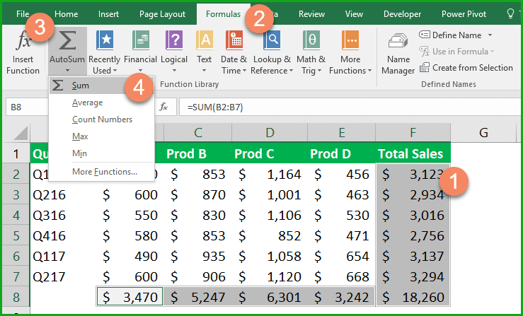
#3. Improve your speed by using Autosum
Autosum is another handy feature when it comes to adding the SUM formula for multiple Columns/Rows.
With the help of this function, you can insert a formula into multiple cells with a single click.
Here is an example of how to get started with excel auto sum functionality.
Alternatively, you can also use the excel keyboard shortcut Alt+Equal for the same.
#4. Customize your Quick Access Toolbar [QAT]
QAT is a customizable toolbar as per the user requirement.
You can add your most-used options like Auto filter, Subtotal, Paste Special, etc. to QAT, and then you can access them quickly either by mouse or by using a shortcut from QAT.
For example, if you want to add Autofilter to QAT you can follow simple steps as per below.
Step-1: Navigate to Data → Filter
Step-2: Right-click on Filter option → Select Add to Quick Access Toolbar
Step- 3: Now locate the filter icon added to QAT and then start using
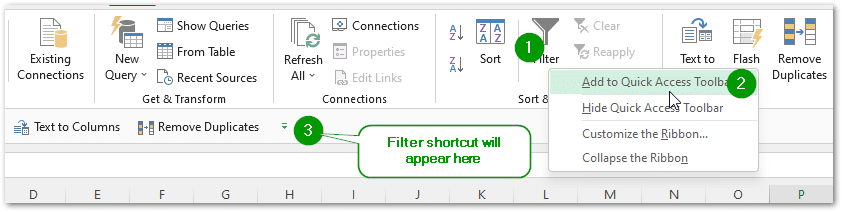
Tip: press the ALT key to find out the keybindings of your QAT shortcuts
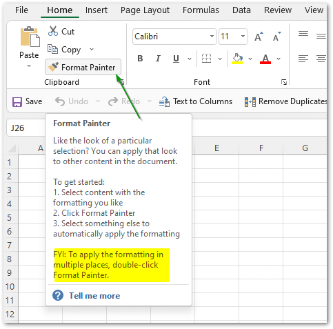
#5. Format Painter
Format Painter is one of my favourite excel tips, it makes our life so much easy to replicate formatting across multiple cells.
With the help of a little tiny painting brush, you can copy formatting from one cell to another cell easily.

With a single click on the format painter icon, you can apply formatting to a single cell, in case if you want to apply for multiple cells then you need to double-click on it.
How to use Format Painter:
- Step1: Select your cell or a group of cells from where you want to copy formating
- Step2: Click on the Format Painter option under the clipboard section [refer below image]
- Step3: Then just place your mouse cursor and click on your destination cell – that’s it
#6. Use wildcards to find & replace data
You can use wildcard characters in excel to find information quickly.
Very often people think this is very difficult and only for advanced users, but the fact is anyone can use it and it works great.
You can use * [Asterisk] to find out any number of characters followed by a specific alphabet.
Alternatively, you can use “? [Question Mark]” for a single character.
For example, if you want to find employee names starting with “Na” you can use Na* you will see results like Nagendra, Nadish, Nakul, etc.
In case you want to find out names starting with N & ending with M you can search like n?????????m. Of course, this is not straightforward.
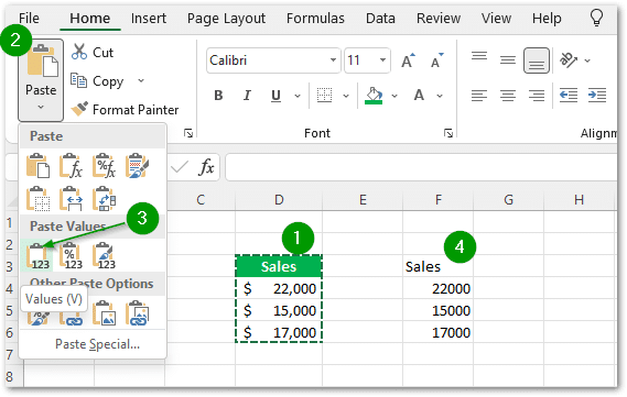
#7. Everything is special with Paste Special
Paste Special is a very unique and useful feature.
Suppose when you want to copy any content from one cell or sheet to another then you are not only copying the content but also the underlying components like formatting (Color, Font, Comments, etc.)
In most cases, you just need the content, not the formatting.
So, to get rid of unwanted formatting simply use the Excel paste special option by pressing Alt+E+S+V to paste values.
Or just follow the below guide.
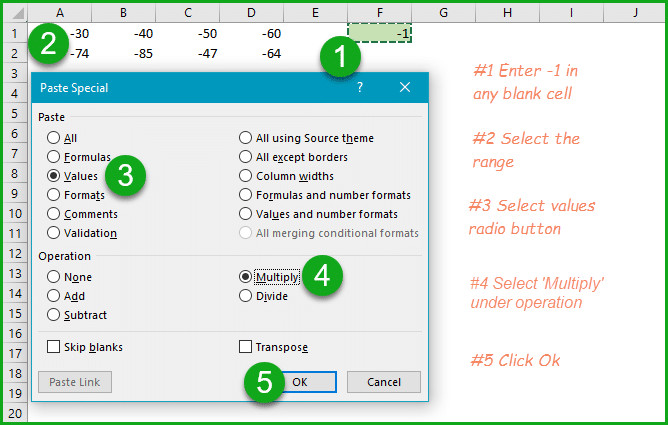
#8. Arithmetic operations with Paste Special
Do you know excel paste special option will support simple arithmetic operations like addition, multiplication, division & subtraction?
I often use these to convert negative numbers to positive with a single click. You can follow the below steps.
It just works great – really good excel tip
#9. Advanced excel tip – Breakdown lengthy formulas
This is one of my favourite excel tips among this list of best excel tips and tricks.
It’s quite evident that we often write lengthy excel formulas to execute complex logic but as you know it’s very hard to debug in case of any errors.
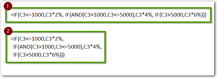
So, the best and the easiest way is to break down formulas by each logic by pressing Alt+Enter in the formula bar.
With the help of the below example, you can see yourself the benefits of breaking down formulas into various lines.
As you can see below the first formula without breaks looks a bit difficult to read and understand but the second one looks much better.
So, just remember this excel tip before you write any complicated formula.
#10. Quick filter technique
There is no doubt, we use excel filters every day.
But I bet 9 out of 10 will not know the quick filter technique that I’m about to show you.
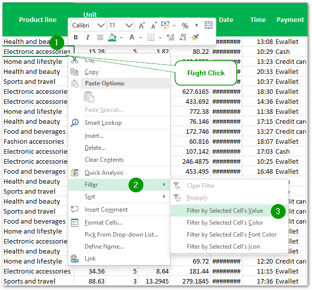
As you can see below, I’m trying to filter data by electronic accessories.
So instead of using the top filter I just need to right-click on electronic accessories and then click on Filter and then Filter by Selected Cells Value.
Now the data will be automatically filtered based on your cell value.
#11. Sort data before working on large files
Large excel files can become a headache very quickly, they will freeze, they will crash and all kinds of issues may crop up.
But you can avoid these issues with a simple excel tip i.e. sorting data before you start working on any excel files.

It works great, I use this excel tip all the time.
The basic purpose of the excel sort function is to organize data as per the commonalities, by doing so excel can apply our various logics quickly in batches.
As a result faster processing time.
#12. Named ranges can add a lot of value
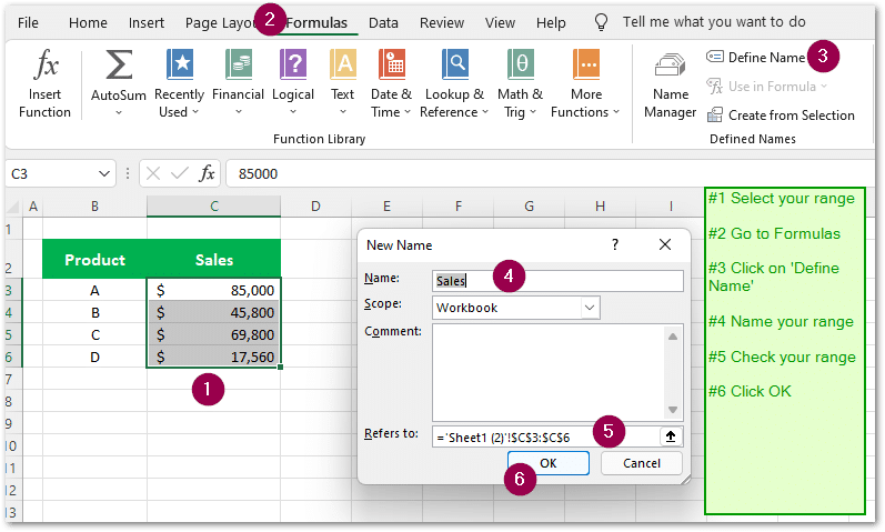
Named ranges play a significant role in the financial modelling world. The more formulas you have in your workbook the more you should use named ranges.
With the help of named ranges, you can assign descriptive names to your ranges and then you can use them in formulas.
Difficult to follow?
You can refer to the below screenshot to learn further on inserting named ranges.
Here is how you can use the named ranges in your formulas.

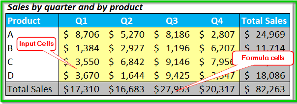
#13. Differentiate Input cells & Formula cells with a colour coding
When we talk about the best excel tips and tricks, colour coding takes centre stage.
It’s a very basic yet most important excel tip for both beginners & advanced users but unfortunately, many will ignore this.
The very basic idea is to separate input cells and formula cells using colour-coding. This will ensure users will not mess up with the formulas.
You may refer to the below example for further understanding.
#14 Control+Enter can solve formula fill problem
Dragging formulas from one cell to another cell is a cool excel tip, but it’s not always advisable. With the help of the CTL+ ENTER combination, you can quickly fill formulas in a selected range.

For example, if you want to add a current date in A1: A5 range:
Select range A1: A5 → enter TODAY() formula → Hit Control+Enter
That’s it, your formula will appear in all the cells.
#15 Never ever hard code your formulas

Admit it!
Hard coding excel formulas will solve your short-term problems, but in a long run, they are extremely harmful, and the worst part is they are very hard to identify.
Here is an example of hardcoded formula.
=A1*1.2%
Just imagine, what will happen if the tax rate changes from 1.2% to 1.5%.
Hence, it’s always a good idea to write formulas that can have cell references so that you can easily modify them in the future.
#16 Hide cell contents in Conditional Formatting
There is no doubt, Conditional formatting plays an important role in data visualization.

But, it’s important that you should know how to hide content in your conditional formatting.
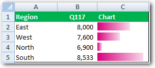
In this example, I’ve used simple data bar formatting to visualize data like below.
Step #1 Copy B2: B5 data and paste it in C2: C5 → Select C2: C5 → Go to Conditional formatting → Data Bars → Choose the one which you like.
Step #2 Again select C2: C5 → Click on Ctrl+1 → Select Custom format → in the ‘type’ field enter ;;; → Click ok
Boom, now you’ll see only formatting like what we have here.
Also read: Building Excel heat maps using Conditional formatting
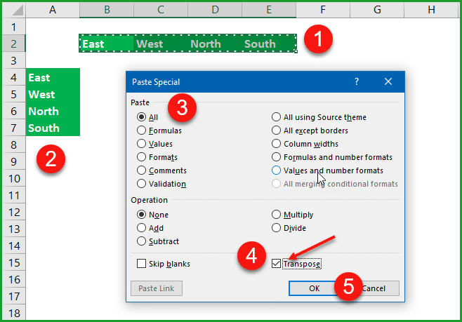
#17 Use Transpose to transform your data
Often messy data will make you struggle a lot.
But with the Excel transpose option, you can pretty much bend your data according to your requirement.
For example, if you want to convert horizontal values into vertical you can follow simple steps as below.
Select & Copy A2: D2 → Click on a blank cell → Alt+E+S+V or Paste special → Select values → enable Transpose check box → Click ok
# 18 Learn CVZY shortcuts to save 90% of your time
CVZY is one of the best excel tips that we all should learn [no exception], it’s hard to imagine how difficult it will be without these.
I know you started guessing, they are
Ctr+c → Copy
Ctr+v → Paste
Ctr+z → Undo
Ctrl+y → Redo
#19 Avoid using Merge & Center
It’s ok to use Merge & Center option for basic needs, but beyond that please try to avoid it.
The main functionality of this option is to combine two or more cells to accommodate data.
But, that comes with a lot of issues.
For example, the cell references will take a hit so as a result most of your formulas won’t work properly.
#20 Beautify your reports with structured formatting

It really matters how you present your data in workbooks. If you just focus on results with some confusing formulas, then your hard work can quickly go unnoticed.
I’d certainly recommend spending a few additional minutes to beautify your workbook.
Having said that, please don’t overdo that, there is a high chance that your workbook may slow down
#21 Use built-in styles for quick formatting
As I mentioned above, formatting is important to present your data.
The funny thing is if you start working on formatting you will tend to spend a lot of time on that because we are colour freaks. The best workaround for this is to start using built-in styles.
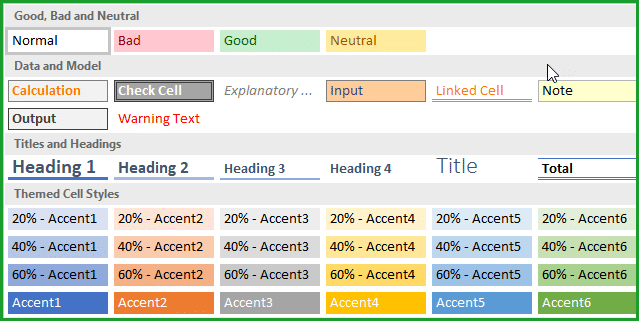
In case if you don’t like built-in styles then create your own styles and use them in your workbook. It’s just a one-time exercise but works like a champ!
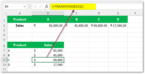
#22 Use Transpose formula for live updates
Using paste special to transpose data is one way, and the other way is to use a built-in transpose formula. If you have live data to be transposed, then the formula will work well.
For example, in the below table Product & Sales columns can be converted to horizontal like below.
As you can see below, the TRANSPOSE formula is surrounded by flower brackets, which means it’s an array formula.
You need to press Control+Shift+Enter to activate array formulas.
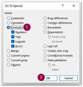
#23 Find & Select (or GoTo special) to identify all the formulas in a worksheet
Do you know with a single click you can find out all the formulas in a worksheet?
Yes, It’s just one click.
With the help of the Find & Select option, you can do that.
Step 1: Press the CTL+G keyboard shortcut
Step 2: Click on the Special button
Step 3: Select the formulas radio button and click OK
Step 4: All your formula cells should have been selected, now you just change the font or fill colour to identify
#24 Be careful with volatile formulas
Using volatile formulas like TODAY, RAND & RANDBETWEEN will have a bigger impact on your workbook performance.
The reason is very simple.
These types of excel formulas will tend to change as and when your workbook refresh happens, and it results in higher processing time.
So, limit using these formulas in your reports/financial models to a minimum.
#25 Calculation Options can help as well as ruin your work
When we talk about the best excel tips and tricks, we certainly need to pay attention to Excel calculation options and their usage.
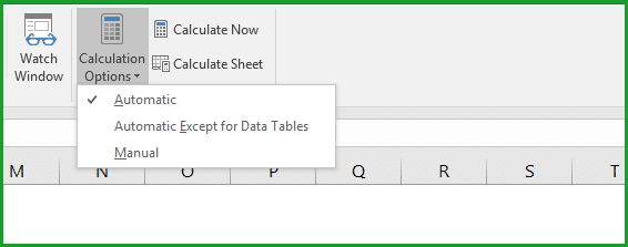
By default, it will be ‘Automatic‘ but you can always change that to ‘Manual‘ to stop calculation until you refresh/save your workbook.
But, you should be very careful while using ‘Manual‘, it can produce incorrect results.
You can access from Formulas → Calculation options → Automatic/Manual
Also read: 10 Reasons for Excel Formulas not Working
#26 best excel tip – GET RID OF GRIDLINES
The is no doubt, gridlines are good for basic reporting.
But, in excel dashboards gridlines aren’t necessary. Your Dashboards will not look clean with the gridlines, hence I’d recommend disabling them.
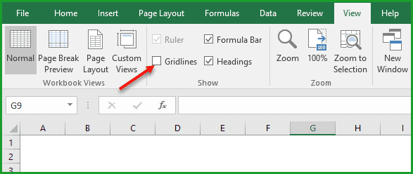
You can disable it from → View → Show/Hide → Uncheck Gridlines checkbox
#27 Use TRIM formula to remove unwanted spaces
Unwanted spaces will make you struggle a lot. Most of your formulas will break because of the useless blank space between words or numbers.
And the worst part is you can’t identify them quickly.
So, use the TRIM formula to remove unwanted spaces in a text like below:
=TRIM(“Hello Good Morning”) = Hello Good Morning
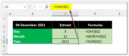
#28 Extract Day, Month & Year from a date
In a typical financial modelling environment, you sometimes need to split days and Months from a full date.
For example, to split Day, Month & Year from 04 December 2021 you can use three simple date formulas like below.
These are simple formulas but trust me they are very handy.
#29 Measure length of a string with LEN formula
LEN is a simple formula to check the length of a text string. This formula will help you identify total letters/words/symbols/spaces in a sentence.
Here is an example:
=LEN(“Best Excel Tips and Tricks”) will return 26, which means we have 26 letters in our text string.
LEN formula alone will not help you much, but when you combine it with other formulas then the results will be amazing.
#30 Use IFERROR formula for error management
How awkward it is to have #N/A, #VALUE, #DIV/0! in complex financial models.
The good news is, there is a way to manage these errors using the IFERROR formula, it’s very simple yet effective. Please refer to the below example for further understanding.

#31 Right formula can extract text from right side
I often use the RIGHT formula for various reasons. With the help of this formula, you can extract text from the right side of the text.
For example, to extract the last name from Walter Perry you can use a RIGHT formula like below:
=RIGHT(“Walter Perry”, 5)
I have written an advanced tutorial on how to extract names in excel using various excel formulas, please refer.
Also read: 19 profound ways to bend your data
#32 Left formula to extract text from Left side
The functionality of the LEFT formula is very identical to RIGHT, the only difference is, the text will be extracted from the left side.
For example, to extract the first name, you can use a left formula like below:
=LEFT(“Walter Perry”,6)
#33 MID formula – extract middle name
Similar to RIGHT & LEFT, the MID formula can help you extract the middle value from a text.
For example, to extract the middle name ‘Anthony’ from Mark Anthony Fernandez, you can write a formula like below:
=MID(“Mark Anthony Fernandez”,6,8)
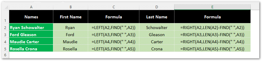
#34 Dynamic Right & Left formulas
When you deal with huge amounts of data, regular Right & Left formulas may not help.
But.. if you combine other simple formulas like LEN & FIND and make it dynamic then they work flawlessly.
You can refer to the below examples:
Of course with the latest excel versions, pattern recognition has become easy.
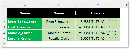
#35 Use SUBSTITUTE formula to replace text
Not many of you know how to use the SUBSTITUTE formula, it’s useful if you know how to use it.
As the name suggests, you can replace a part of the text or full text using the above formula based on a condition.
It works like a FIND & REPLACE function but you can use it for complicated problems by defining the pattern.
For example, to replace underscore between first and last name with space, we can write a formula like below:
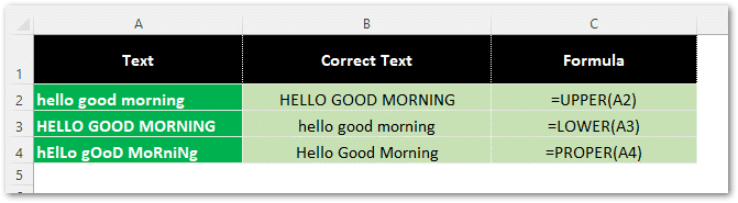
#36 Make use of Upper, Lower & Proper functions to play with the text
There is no better way to handle data in excel other than using text functions:
For example, to convert text from Lowercase to upper case, you can use the UPPER formula, similar to that you can use the LOWER formula for lower case.
And, in case your data is not in a proper format like jumbled with capital & small letters, you can use the PROPER function: refer to the below examples.
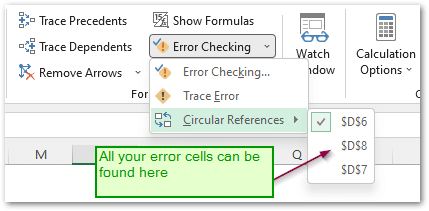
#37 Be careful with circular reference errors
Circular reference errors are the most annoying ones in Excel.
The worst part is, you don’t get to see them quickly, but there is a way to identify these types of errors using built-in options like below.
Go to Formulas tab ==> Formula Auditing ==> Click on Error Checking dropdown ==> Select Circular References
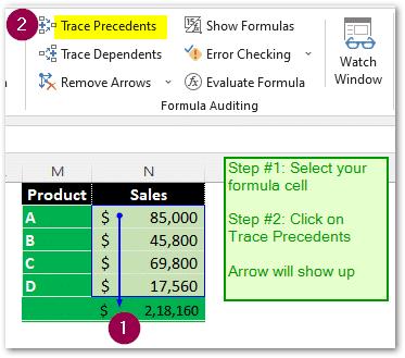
#38 Trace precedents
You can audit formulas in excel using the Trace Precedents option. This will help to identify formula dependencies.
This will come in handy before you delete or alter any formulas to assess the impact.
Place cursor on a formula cell → Formulas → under formula auditing → Click on Trace Precedents
That’s all, now you will see a blue arrow pointing all the precedent cells for a formula.
#39 Trace Dependents
This feature is exactly the other way around to Trace Precedents.
With the help of this, we can easily trace the dependent cells based on the selected cell
Place cursor on a formula cell → Formulas → under formula auditing → Click on Trace Dependents
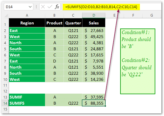
#40 BEST EXCEL TIPS – Take full advantage of Sumif & Sumifs
Financial Modeling is incomplete without SUMIF & SUMIFS formulas.
Be prepared to answer questions like, what was our total sales from South region? what was it during last year same quarter etc.
With the help of simple SUMIF& SUMIFS formulas, you can do pretty much everything.
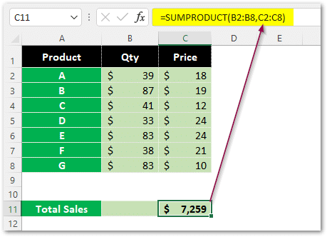
#41 Boost your analytical skills with SUMPRODUCT formula
This one is top-rated in my best excel tips and tricks tutorial.
I’m sure most of us don’t use the SUMPRODUCT formula very often.
Let’s be honest, we don’t use it because we don’t know how to use it, trust me I was also on that list.
With the help of the SUMPRODUCT formula, you can easily calculate the cumulative sum. It will be very quick and save quite a bit of time.
Refer to the below example to understand further.
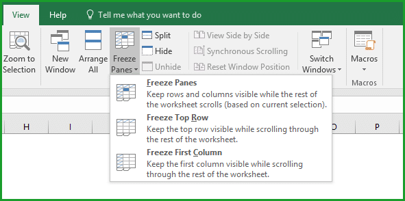
#42 Don’t scroll Up & Down, use Freeze Panes
Scrolling up & down will ruin your time.
Instead, you can use the Freeze Panes option to make your headers constant.
You can find this option under → View → Freeze Panes
#43 Generate Random numbers using Randbetween formula (Caution)
With the help of the RANDBETWEEN formula, you can generate random numbers very quickly. The good news is, you can specify your upper & lower limits.
In fact, most of the examples for this article have been generated using this formula.
For example, If you have to generate 4 digit numbers, you can write a formula like the below:
=RANDBETWEEN(1000,9999)
Caution: Please make sure to convert RANDBETWEEN formula cells to values, otherwise the numbers will change every time you save/refresh your workbook.
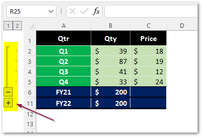
#44 Use ‘Group’ feature to organize your workbook
Perhaps grouping is one of the very old excel features but an extremely powerful excel tip.
You can systematically organize your workbook data by grouping them together.
To access this option navigate to Data → under Outline → Group or Ungroup
Alternatively, you can also use excel shortcut key → Shift + Alt + Right Arrow
#45 Excel tip for spead – Be a keyboard user
After all, timing is everything.
Sending reports after the deadline is almost equal to not sending.
You can save a lot of time by using keyboard shortcuts, you don’t need to learn all of them you just need a few, just start learning
#46 Commenting is essential – yet we ignore
We often work with a bunch of excel formulas to get things done.
Indeed, it works.
But, what if you have to revisit your calculations after a week or a month?
It’s disgusting! because you forgot what you had worked on and sadly you don’t have any notes to refer.
That sounds like a familiar incident, right?
To avoid this, you can simply use the built-in comment feature to document your manual adjustments, important points & supporting notes, etc.
You can insert a comment by right-clicking on a cell → Select Insert Comments option
#47 “Prepare for Tsunami” – Always backup your workbooks
Excel is your Friend as well as Foe.
Excel is your best friend, based on the rich functionalities to get things done, at the same time it can quickly ruin your hard work in a way of crash or corrupt workbooks.
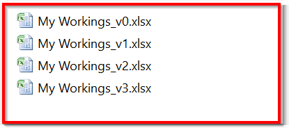
So, the best practice is to adopt a backup method.
I personally use the ‘Version control method’, trust me it’s very simple.
Just do Save as after major changes and add suffix as v1, v2 v3…etc to the file name.
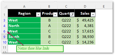
#48 Quick filter check
Sometimes it’s a bit difficult to check whether the filter is applied in your workbook or not. Often you may have tried completely taking off the filter for confirmation.
But, you can quickly check by referring to left-side row numbers.
In case the filter is on, then you will see row numbers are highlighted in Blue (similar to a hyperlink).
Nice excel tip isn’t it?
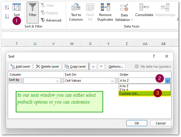
#49 Use custom sort – cool excel tip
Most of you limit yourself to the ‘A to Z & Z to A Sorting’ method.
But, you have got a lot of sorting options, like Sort by font colour, sort by fill colour & sort by icons, etc.
You can even define your own sorting method as per your requirement – refer to the below example.
#50 Spell check works in Excel too
It’s quite evident that spell checks integrated very well into MS Word than Excel.
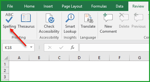
But, you can still use the same feature in excel as well.
You can access the spell check feature from Review → Spelling, alternatively, you also can use the F7 shortcut key.
#51 Don’t let someone ruin your hard work – Protect your formulas
Formula protection is a key aspect of financial modelling, it’s important to safeguard some of your critical formulas.
You can do this by simply defining which cells users can edit/formula cells that you want to hide from view. Follow simple steps to hide formulas.
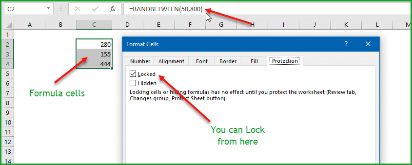
Step#1: Control+A to select entire sheet range → Click on format cells → Go to protection tab → make sure to disable ‘Locked’ & ‘Hidden’ checkboxes → Click ok.
Step#2: Select a formula cell → Right Click → Format cells → Protection → to enable ‘Locked’ & ‘Hidden’ checkboxes → Click on ok.
Step#3: Go to Review Tab → Click on Protect sheet → If you want you can provide Password, if not click on Ok.
That’s it.
Conclusion – Best Excel Tips and Tricks
We deliberately did not include Vlookup, Match & Index formulas in our best excel tips and tricks list.
I feel these two formulas are very broad to cover, thus it’s good to have a separate tutorial than a small paragraph. I have already written an in-depth tutorial on Vlookup you may refer to that link.
Now, it’s your turn! do you think I have missed any of your best excel tips and tricks? If so, please comment below.
Icons credit: flaticon.com